5 Strings and tidyr
First step: let’s load in the data and required packages. This is the standard McMurray & Jongman dataset of fricative and vowel measures that we’ve been using this term.
5.1 Working with character strings
In R, we frequently have to process strings of text to create new variables. We’ve come across this previously with the substr() function when we had to extract the “M” or “F” part of a participant’s ID to create a column for their gender. We’ll learn some of these functions a little more formally in this section.
5.1.1 Substrings: substr()
The substr() function extracts a substring from some character variable. It takes three arguments: the character vector you want to operate on, the starting character number, and the ending character number.
5.1.2 Concatenating strings together: paste() and paste0()
The functions paste() and paste0() let you paste two strings together. paste0() simply pastes together whatever strings you feed it with no separation between them. paste() is a little more flexible and allows you to specify the separator using the sep() argument. You can put as many strings as you want in the argument slots to paste them together.
5.1.3 Regular expressions
Regular expressions are character sequences that form a search pattern, and are a common component of programming languages. (Even Praat has regular expressions.) They are very useful when you might need to target a class of characters instead of an exact instance. The square brackets contain the class of characters you might want to target; there are also some symbols for indicating things like “must occur at the beginning of the string” or “must occur at the end of the string” or “must occur at least one time”. Here are some useful regular expressions in R:
- [A-Z] or [[:upper:]] = all uppercase letters
- [a-z] or [[:lower:]] = all lowercase letters
- [A-Za-z] or [A-z] or [[:alpha:]] = all letters
- [aeiou] = the letters a, e, i, o, or u
- [0-9] or [[:digit:]] = all digits
- [0579] = the digits 0, 5, 7, or 9
- [A-z0-9] or [[:alnum:]] = alphanumeric letters
- * = matches at least 0 times
- + = matches at least 1 time
- [^ ] = does not match one of these strings
- ^[ ] = matches the start of a string
- [ ]$ = matches the end of a string
We can use these regular expressions now in any functions that operate on character vectors. We’ll discuss pattern matching functions with grep() and grepl() and a substitution function, gsub(). Several other functions that operate on character vectors exist, but I personally tend to use these the most (alongside substr()). You should at this point start imagining how you can use these functions that work on characters in combination with other functions like filter() or subset(), etc.
5.1.4 Pattern matching with regex: grep() and grepl()
To identify strings that match some pattern, we can use grep() and grepl(). As copied from the help page on these functions, grep() and grepl() “search for matches to an argument pattern within each element of a character vector.”
grep() tells you which indices contain matches.
grepl() tells you, for every index in the vector, whether a match is TRUE or FALSE. (The l stands for logical, so it gives you a TRUE/FALSE statement for every index.)
grep() and grepl() both take two main arguments: the pattern you want to match on and the character vector to look in.
tmp <- grep("f", mcm$Fricative)

tmp2 <- grepl("f", mcm$Fricative)

animals <- c("cats", "dogs", "mice", "chickens", "geese", "birds")

contains_twoplus_vowels <- subset(animals, grepl("[aeiou][aeiou]", animals))

reg_plural <- grep("s$", animals)
reg_plural2 <- grepl("s$", animals)
reg_plural_animals <- subset(animals, grepl("s$", animals))

# NEGATION
irreg_plural_animals <- subset(animals, !grepl("s$", animals))
5.1.5 Substitutions with regex: gsub()
Another common function that manipulates character vectors is gsub(), which is for string substitution. I frequently use this if I have, for example, a very long participant or file ID, and that ID contains some important information and some useless information. I might split the ID up by deleting or replacing the unrelevant parts.
gsub() takes three arguments: the string to be replaced, the string to replace it, and the character vector to operate on
5.2 Data formatting
5.2.1 Merging datasets
It’s frequently useful to be able to merge two separate datasets into one. We’ve needed to do this in the past, but have used cbind() which just pastes the two datasets together by columns. Ideally, though, we’d merge the two datasets on one or more variables, which makes sure that like rows match up with like rows, even if it’s out of order. The variables you merge on act like a unique identifier for the row.
For example, last week we ran the following code as setup for the correlation:
spkr_vowel_means <- mcm %>%
  group_by(Talker, Vowel) %>%
  summarise(mean = mean(dur_v, na.rm = T))

spkr_mean_a <- subset(spkr_vowel_means, Vowel == "a")
spkr_mean_i <- subset(spkr_vowel_means, Vowel == "i")

vdur_ai <- cbind(spkr_mean_a$mean, spkr_mean_i$mean)
colnames(vdur_ai) <- c("mean_vdur_a", "mean_vdur_i")
vdur_ai <- data.frame(vdur_ai)
We can instead use the merge() function to join spkr_mean_a and spkr_mean_i together. The merge() function takes three arguments: the two datasets you want to merge, and a vector of the column names you want to merge on. You can technically merge columns that have different names in different datasets, but in this case, the column name for the common column is the same: “Talker”. In addition, there is only one common column:
spkr_vowel_means <- mcm %>%
  group_by(Talker, Vowel) %>%
  summarise(mean = mean(dur_v, na.rm = T))

spkr_mean_a <- subset(spkr_vowel_means, Vowel == "a")
spkr_mean_i <- subset(spkr_vowel_means, Vowel == "i")

vdur_ai <- merge(spkr_mean_a, spkr_mean_i, by = "Talker")
Note how there is only one Talker column. Annoyingly, the distinct Vowel and distinct mean columns had the same names so those are now Vowel.x and Vowel.y, etc. We can go through and clean up the names using the colnames() function:
5.2.2 Wide format data, long format data, and tidy data
Wide format data refers to a spreadsheet where a single row contains multiple columns for related attributes of a single data point / subject. For example, each column could be the response value for a trial in an experiment. I am pretty sure it is the default output of Qualtrics, which many of you will be using for your dissertation. As the name suggests, it is wide in appearance.
Long format data refers to a spreadsheet where one column specifies the attribute of a data point and another column specify the value of that attribute. Trial number/type would be listed in one column and the response value for that particular trial would be listed in another column. Subject information is frequently repeated across many rows. As the name suggests, it is long in appearance.
Datasets are frequently a mix of the two types, such as the McMurray & Jongman fricative dataset we’ve been using. It’s long format in the sense that we have multiple rows for each subject, but it’s wide in that several attributes of the measured fricative are spread across several columns. Though it’s a mix, the McMurray & Jongman fricative dataset is considered to be a tidy dataset.
Tidy datasets have one observation per row, one column per variable, and one table for observational unit. That last part means that all of the observations coming from one source (e.g., a participant) are grouped together in the dataset.
Tidy datasets are easiest to work with in R, but it’s not always the case that you will start with a tidy dataset. Sometimes you’ll have to spend some time to get it in the proper format (e.g., working with Qualtrics output).
Certain analyses and plots also frequently require the dataset to either be in wide or long format. For example, analyses or plots that require within-subject comparisons such as correlations or paired t-tests on subject means require wide format data: one column for each condition that will then be compared. Long format data is sometimes required for certain ggplots when you want to map an attribute of the data point to some aesthetic.
You don’t want to overthink this too much, but if you find yourself stuck in getting an analysis to work, you might have to pivot some part of the dataset to either long or wide format. To do this, we’ll use the pivot_longer() and pivot_wider() functions in the tidyr package of the tidyverse.
5.2.3 Wide to long (and tidy) format using tidyr
In this example, we’ll be working with a wide format dataset: accentRecog_resp.csv. This is a fake dataset modeled after the output of a Qualtrics experiment testing accent recognition.
The goal is to convert this to a tidy dataset with one observation per row, one column per variable, and one table for observational unit.
Take a look at the dataset and note the wide format: each column is a unique trial for a given participant. We first need to project the trials into a single column and have a new column specifying the attributes of the trial in the column after it. To do this, we use the function pivot_longer().
accentRecog <- mydata %>% pivot_longer(cols = starts_with("q"), names_to = "trial", values_to = "langResp")Or equivalently:
accentRecog <- mydata %>% pivot_longer(-c(subj, nativeLang), names_to = "trial", values_to = "langResp")In the second function, I am subtracting or “deselecting” certain columns that should effectively stay put – they should not be regrouped or changed in any way. Notice how now there is one row per trial and multiple rows grouped together for subject.
5.2.4 Long to wide format using tidyr
In this example, we’ll be working with our regular mcm dataset, and running our regular group_by()-summarise() sequence on the individual speakers and fricatives to get speaker mean durations for each fricative
Take a look at the created dataset and note the long format: the first two columns specify the attributes belonging to the value in the third column, where the value here is the mean fricative duration. This is technically tidy already, but you’ll frequently find that you need the wide format for certain operations. We’ll convert this to wide format where the levels of the fricative category each have their own column with the corresponding mean duration in each; the talker column will basically stay the same but shorten to accommodate the reduced length. To do this, we use the function pivot_wider().
In the function, we use the names_from argument to refer to which column contains the names that should become the new column names. The values_from argument refers to which column contains the values that should fill the cells of those new columns. Note the difference in the use of quotations between pivot_longer() above and pivot_wider() here. In the tidyverse style of code, when we are creating a new column, we use quotes; when we are referring to an existing column, we leave it unquoted.
5.3 Practice
- Import mandarinVOT.csv. The first column contains the filenames of the audio files from which VOT measurements were extracted. The filename has the following structure:
“ALL_005_M_CMN_CMN_DHR_autovot”
- ALL: ALLSSTAR corpus
- 005: speaker ID (always three numbers)
- M: gender (can be M or F)
- CMN: language spoken in the audio file (always three uppercase letters)
- CMN: first language (always three uppercase letters)
- DHR: task ID (always three characters but can be letters or numbers: e.g., DHR, LPP, HT1, HT2)
- autovot: refers to the program used to process the wav file; not relevant for any analysis
Create a unique column for each of the following: the corpus, the speaker ID, the gender, the language spoken in the audio file, the speaker’s first language, and the task ID. For the speaker ID, you should also add a character prefix to the digits like “s” or “subj” so that R doesn’t misinterpret the ID as an actual number (e.g., it should be “s005”, not “005” for the above speaker). (Please also ignore the fact that the corpus is always ALL and the languages are always CMN, or Mandarin Chinese. For the sake of practice, pretend as if they might vary.)
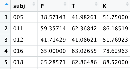
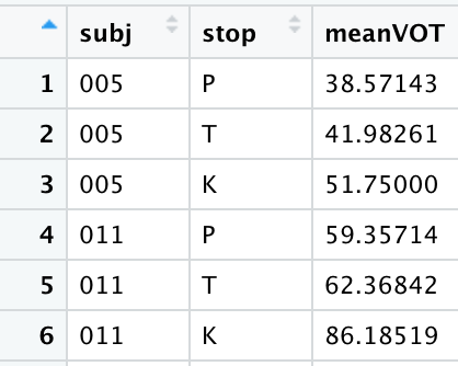
Run the following code for obtaining talker- and stop-specific VOTs:
Now pivot this dataset to make it wider. There should be 4 columns: one for the speaker (that doesn’t change), and now three columns for P, T, and K, that should contain the talker-specific VOTs. You’re essentially spreading out the stop column and filling in the values from the meanvot column.
- Take the generated dataset in (3) and convert it back to long format using pivot_longer()